Now let us imagine that we need to find the boundary between dark and light regions.
For a human, this is obvious: it is enough to look at the image. But a computer must perform certain calculations to detect such a change in brightness.
One way to solve this problem is to use a small weight matrix called a convolution kernel (kernel).
It moves across the image, analyzes small patches of pixels, and calculates how much they differ from one another.
This is the mechanism we will examine next.
2. What Is Convolution (Convolution)
Convolution is an operation in which a small weight matrix moves across an input matrix. At each position, corresponding elements of the two matrices are multiplied, and the results are then added together.
The weight matrix is called a convolution kernel (kernel), and the result of applying the kernel to all valid positions of the input is a feature map (feature map).
Let us look at how this works in practice.
Convolution Kernel
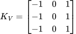
Suppose we have an image represented by a matrix of numbers. To find vertical edges in it, we will use a 3 × 3 filter:
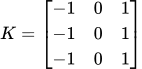
The negative weights are on the left, and the positive weights are on the right.
This arrangement is not accidental. The filter compares the brightness of the left and right parts of a small region of the image.If the values on the right differ significantly from those on the left, the result of the calculation will have a large absolute value.
If both parts have approximately the same brightness, the positive and negative terms will cancel each other out.
Sliding Window
Now imagine that we overlay our kernel onto the image.
The filter covers a 3 × 3 region and performs a calculation. It then moves one position to the right and repeats the operation.
When it reaches the right edge, it moves to the next row.
Thus, the filter sequentially processes all valid regions of the image.
Each calculation produces one number. By collecting all the resulting values, we obtain a new matrix—a feature map (Feature Map).
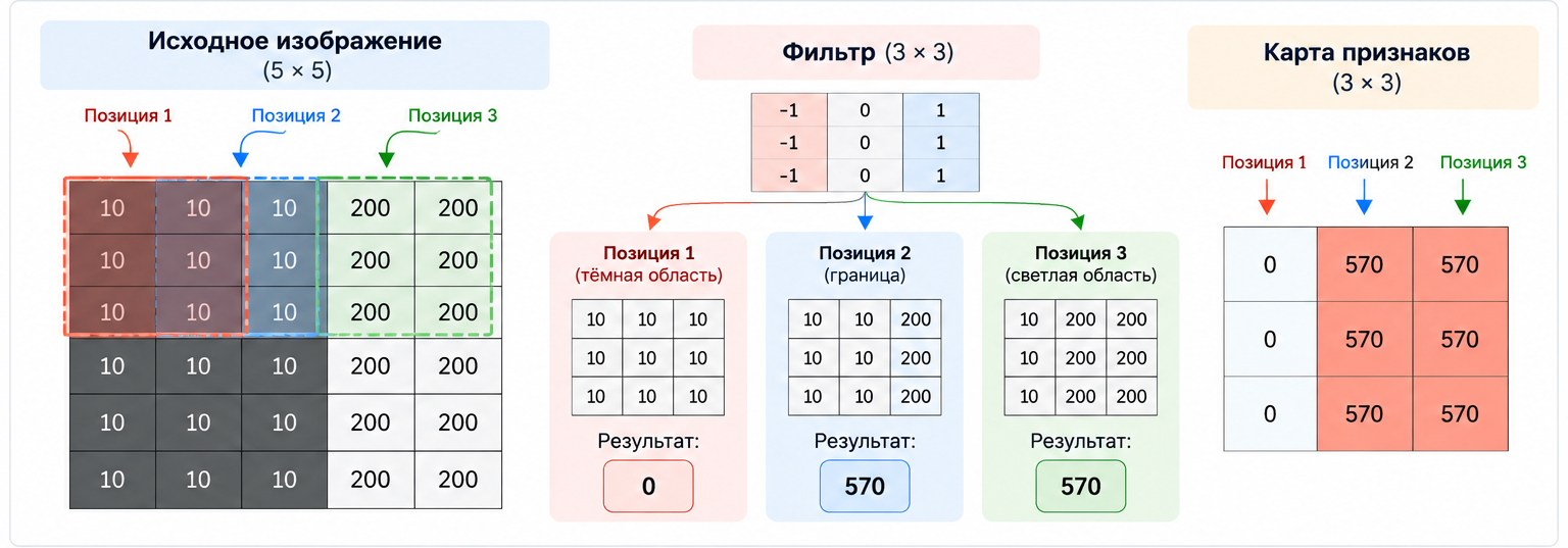
Let’s look at one calculation
Let’s take a small region of the image:
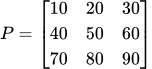
And apply our kernel to it:
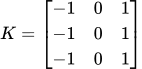
Multiply the elements located at corresponding positions and add the results:
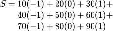
We get:

The result is 60.
This number becomes one element of the output feature map. The filter then moves to the next position, and the calculation is repeated.
Convolution or Cross-Correlation?
There is a small technical subtlety.
In mathematics, the convolution operation assumes that the kernel is first flipped by 180 degrees.However, most implementations of convolutional layers in neural networks use a different operation—cross-correlation—in which the kernel is applied without flipping.
This is the variant we will use in our PHP program.
In the context of deep learning, this operation is also usually called convolution.
What do we get?
After the filter has processed the entire image, we will obtain a new matrix—a Feature Map.
It shows how strongly the selected filter responds to different parts of the image.
Large positive or negative values indicate a strong filter response, while values close to zero indicate the absence of a pronounced feature that the filter is looking for.
Now that we have understood how convolution works, we can move on to the implementation. Let us try writing this operation ourselves in PHP and check whether our filter can indeed detect vertical boundaries.
3. Implement convolution in pure PHP
Now that we have understood how convolution works, let us try implementing it ourselves.
We will not need third-party libraries, ready-made ML algorithms, or specialized image-processing tools. Plain PHP and a few nested loops will be enough.
Prepare the input data
First, let us create a small 5 × 5 image. As before, we will represent it as a two-dimensional array of numbers.
The left side of the image will be dark and the right side will be light:
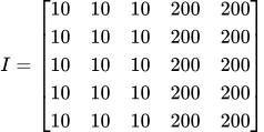
A vertical boundary lies between the third and fourth columns.It is exactly this that we want to detect.
Now let's define the convolution kernel:
Negative weights on the left and positive weights on the right allow the filter to respond to brightness differences between the left and right parts of the area being processed.
Our implementation will use the following settings:
stride = 1 — the filter moves one pixel at a time;
padding = 0 — no additional pixels are added along the edges;
the kernel is not flipped;
the result values are not limited to the range from 0 to 255.
TAG120@@(
 and (
 ) are the width and height of the input matrix;
(
 ) and (
 ) are the width and height of the kernel.
a positive result corresponds to a transition from a dark region to a bright one from left to right;
a negative result corresponds to a transition from a bright region to a dark one from left to right.
Different filters respond to different directions of brightness change.
Changing the signs of the weights changes the sign of the response.
Reducing the contrast leads to a decrease in the absolute magnitude of the response.
The same filter can produce a strong response at several neighboring positions.
The last point is especially important. Feature Map values are the results of mathematical calculations, not the original pixel values. Therefore, they may be negative or exceed 255.
Let's write the convolve() function
Let's create a convolution.php file and implement the convolve() function.
It will accept two two-dimensional matrices: the input data and the convolution kernel. The output will be a new matrix—a feature map.
To begin with, let's make the implementation generic: it will support rectangular matrices and kernels of arbitrary size.
/** * Apply a convolution-style filter to a 2D matrix. * * This implementation uses cross-correlation: * the kernel is not flipped. * * @param array<array<int|float>> $input * @param array<array<int|float>> $kernel * @return array<array<int|float>> */ function convolve(array $input, array $kernel): array { if (!array_is_list($input) || !array_is_list($kernel)) { throw new InvalidArgumentException('Input matrix and kernel must use sequential numeric indexes.' ); } $inputHeight = count($input); $inputWidth = count($input[0] ?? []); $kernelHeight = count($kernel); $kernelWidth = count($kernel[0] ?? []); if ($inputHeight === 0 || $inputWidth === 0) { throw new InvalidArgumentException('Input matrix must not be empty.'); } if ($kernelHeight === 0 || $kernelWidth === 0) { throw new InvalidArgumentException('Kernel must not be empty.'); } foreach ($input as $row) { if (!array_is_list($row) || count($row) !== $inputWidth) { throw new InvalidArgumentException( 'Input matrix must be rectangular.' ); } } foreach ($kernel as $row) { if (!array_is_list($row) || count($row) !== $kernelWidth) { throw new InvalidArgumentException( 'Kernel must be rectangular.' ); } } if ($kernelHeight > $inputHeight || $kernelWidth > $inputWidth) { throw new InvalidArgumentException( 'Kernel must fit inside the input matrix.' ); } $outputHeight = $inputHeight - $kernelHeight + 1; $outputWidth = $inputWidth - $kernelWidth + 1; $output = []; for ($y = 0; $y < $outputHeight; $y++) { $outputRow = []; for ($x = 0; $x < $outputWidth; $x++) { $sum = 0; for ($ky = 0; $ky < $kernelHeight; $ky++) { for ($kx = 0; $kx < $kernelWidth; $kx++) { $pixel = $input[$y + $ky][$x + $kx]; $weight = $kernel[$ky][$kx]; $sum += $pixel * $weight; } } $outputRow[] = $sum; }$output[] = $outputRow; } return $output; } /** * Print a matrix in a readable format. */ function printMatrix(array $matrix): void { foreach ($matrix as $row) { echo implode("\t", array_map( static fn (int|float $value): string => (string) $value, $row )) . "\n"; } }Now let's add the original image and the kernel:
$image = [ [10, 10, 10, 200, 200], [10, 10, 10, 200, 200], [10, 10, 10, 200, 200], [10, 10, 10, 200, 200], [10, 10, 10, 200, 200], ]; $verticalEdgeKernel = [ [-1, 0, 1], [-1, 0, 1], [-1, 0, 1], ]; echo "Input image:\n"; printMatrix($image); echo "\nVertical edge kernel:\n"; printMatrix($verticalEdgeKernel); echo "\nFeature map:\n"; $featureMap = convolve($image, $verticalEdgeKernel); printMatrix($featureMap);Let's break down how the function works
Now let's look at the main parts of the implementation.
1.We calculate the size of the output matrix
Since we do not use padding, the filter can process only those regions that fit entirely within the original image.
Therefore, the result dimensions are determined by the formulas:


Here:
In our example, the input matrix is 5 × 5, and the kernel is 3 × 3.
Therefore:

The resulting matrix will have a size of 3 × 3.
2. Moving the filter across the image
This is handled by two outer loops:
for ($y = 0; $y < $outputHeight; $y++) { for ($x = 0; $x < $outputWidth; $x++) { // Process the current image region } }The $y variable determines the row, and $x determines the column in which the top-left corner of the filter is located.
At each position, the kernel processes a 3 × 3 image region.
3. Multiplying the corresponding elements
Inside the outer loops, there are two more loops:
for ($ky = 0; $ky < $kernelHeight; $ky++) { for ($kx = 0; $kx < $kernelWidth; $kx++) { $pixel = $input[$y + $ky][$x + $kx]; $weight = $kernel[$ky][$kx]; $sum += $pixel * $weight; }}Here, the main work is performed.
We take the next pixel from the current region of the image, multiply it by the corresponding kernel weight, and add the result to the $sum variable.
After all kernel elements have been processed, $sum contains the final value for the current filter position.
4. Save the result
Once processing of the current region is complete, we add the resulting value to the output row:
$outputRow[] = $sum;After processing the entire row, we add it to the resulting matrix:
$output[] = $outputRow;Once the filter has processed all valid positions, the function will return the completed Feature Map.
Thus, the entire convolution operation is implemented using four nested loops: two are responsible for moving the filter, and the other two for performing calculations within the current region of the image.
4. Run the program and analyze the result
The convolve() function is ready. Now let's run the program and see what feature map it builds for our image.
Run the following command:
php convolution.phpWe will get the following result:
Input image: 10 10 10 200 200 10 10 10 200 200 10 10 10 200 200 10 10 10 200 200 10 10 10 200 200 Vertical edge kernel: -1 0 1 -1 0 1 -1 0 1 Feature map: 0 570 570 0 570 5700 570 570As a result, instead of the original 5 × 5 matrix, we obtained a new 3 × 3 matrix.
Note that the first column of the feature map contains zeros, while the next two contain large positive values.
This is exactly the behavior we expected from the selected filter.
But why did we get this particular feature map? Let’s manually examine several positions of the filter.
Position 1. Uniform dark region
Let’s start with the first region of the image:
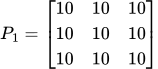
Apply our kernel to it:
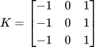
Calculate the result:
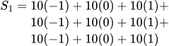 All terms cancel each other out:
 The filter detects no change in brightness from left to right, so the result is zero.TAG271@@Position 2. Transition from a dark region to a light region
Now move the filter to the right. It will cover the region:
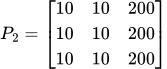 TAG276@@For each row, the calculation is the same:
 TAG279@@Since the filter has three identical rows, we add the three results:
 TAG282@@We get:
 TAG285@@The filter detects a significant change in brightness from left to right.TAG287@@Position 3.The next section with a brightness transition
Let’s move the filter one more position to the right:
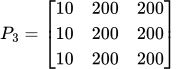
For each row: 
Final value: 
The result is again 570.
Why does a single boundary produce two responses?
There is an interesting point here.
It may seem that two positive values in the feature map indicate the presence of two separate boundaries. But that is not the case.
Both results arise from the same transition between the dark and light regions.
The point is that the filter responds to the difference between the left and right columns of its window. Therefore, a strong response persists in two adjacent positions: in both cases, the window captures pixels from the dark and light regions.
This is normal behavior for the chosen kernel, not an implementation error.
Thus, we have not merely obtained a new matrix of numbers. We have seen how the filter responds to a specific image structure and transforms it into a feature map.
In the next experiment, we will try changing the kernel and see how this affects the result.
5. Experimenting with Filters
Until now, we have used a single filter that detects changes in brightness from left to right. But what will happen if we change its weights?
Let’s conduct several experiments on the same image.
5.1.We are looking for horizontal edges
In the previous example, our kernel responded to changes in brightness from left to right.
Now let’s try detecting changes from top to bottom.
To do this, let’s change the arrangement of the weights:
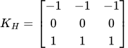
The negative weights are at the top of the kernel, and the positive weights are at the bottom.
Now the filter compares the upper and lower parts of each region of the image.
Let’s add a new kernel to the program:
$horizontalEdgeKernel = [ [-1, -1, -1], [ 0, 0, 0], [ 1, 1, 1], ]; $featureMap = convolve($image, $horizontalEdgeKernel); echo "Horizontal edge feature map:\n"; printMatrix($featureMap);Let’s run the program.
Result:
0 0 0 0 0 0 0 0 0Why are all the values zero?
Let’s look at our original image. All its rows are identical: the brightness does not change from top to bottom.
Therefore, the upper and lower parts of each region contain the same values. The positive and negative terms cancel each other out.
This means that the selected filter did not detect any changes in brightness from top to bottom.
5.2. Changing the filter direction
Let’s return to detecting vertical edges.
In the original kernel, the negative weights were on the left and the positive weights were on the right:
Now let’s change the signs of all the weights:
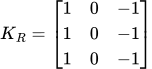
In PHP, it looks like this:
$reverseVerticalKernel = [ [ 1, 0, -1], [ 1, 0, -1], [ 1, 0, -1], ]; $featureMap = convolve($image, $reverseVerticalKernel);echo "Reverse vertical edge feature map:\n"; printMatrix($featureMap);Now the result will be different:
0 -570 -570 0 -570 -570 0 -570 -570Note: the absolute values remained the same, but the sign changed.
Why?
Because now the positive weights are on the left, and the negative weights are on the right.
Thus, the filter responds not only to the presence of an edge, but also to the direction of the brightness change.
In our example:
If we are interested in the strength of the response regardless of direction, we can use the absolute value of the result.
5.3. What will happen if we reduce the contrast?
Now let's conduct one more experiment.
Previously, the brightness of the dark region was 10, and that of the bright region was 200.
The difference between them was: 
Let's try reducing the contrast of the image. To do this, replace the values of the bright pixels from 200 with 100:
$image = [ [10, 10, 10, 100, 100], [10, 10, 10, 100, 100], [10, 10, 10, 100, 100], [10, 10, 10, 100, 100], [10, 10, 10, 100, 100], ]; $featureMap = convolve($image, $verticalEdgeKernel); echo "Feature map with lower contrast:\n";printMatrix($featureMap);Now the brightness difference is: 
Let’s look at the result:
0 270 270 0 270 270 0 270 270The response decreased from 570 to 270.
This is expected: the filter computes a weighted sum of pixel values. When the difference between the dark and light regions becomes smaller, the result of the calculation also decreases.
Thus, we see that the magnitude of the response depends not only on the position of the boundary, but also on the contrast between neighboring regions.
What did our experiments show?
We used the same image, but varied the kernels and pixel values.
As a result, we observed several important features:
This is why multiple filters are used in convolutional neural networks. Each of them can respond to specific features of the input image.
However, in our example, all the weights are set manually. In a real CNN, the network learns to select them on its own during the training process.
Let’s examine how our implementation relates to the operation of convolutional neural networks.
6.How is this related to convolutional neural networks?
At first glance, it may seem that we have simply written a small image-processing algorithm. But it is precisely the operation we implemented that underlies the convolutional layers of a CNN.
The difference lies in where the filter weights come from.
In our program, we manually specified the kernel:
$verticalEdgeKernel = [ [-1, 0, 1], [-1, 0, 1], [-1, 0, 1], ];We already knew which feature we wanted to detect and selected the appropriate values ourselves.
In a convolutional neural network, everything works differently.
Instead of a single predefined filter, the network uses multiple filters. Each has its own set of weights and produces its own feature map.
During training, the values of these weights are adjusted so that the network can better solve the task at hand.
For example, one filter may learn to respond to vertical edges, another—to horizontal ones, and a third—to specific textures or other local structures.
At the same time, we do not need to tell the network in advance which features it should look for.It learns to identify useful patterns based on training data.
What happens inside a convolutional layer?
The process can be simplified as follows:
An image is fed in as input.
The convolutional layer applies several filters to it.
Each filter produces its own feature map.
During training, the network adjusts the filter weights, reducing the prediction error.
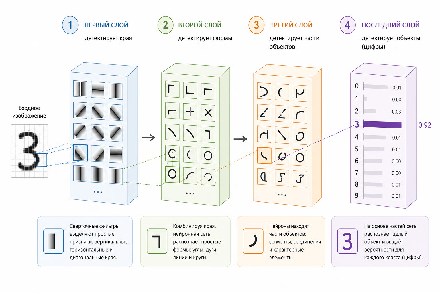
Several convolutional layers can successively extract increasingly complex features.
For example, the first layers may respond to simple structures such as edges, lines, and textures. Deeper layers may combine these features into more complex visual representations.
Why does this work more efficiently than fully connected layers?
One important feature of CNNs is the reuse of the same filter weights in different parts of the image.This principle is called Weight Sharing (weight sharing).
Instead of creating separate weights for each pixel and each position, the network applies the same kernel to the entire image.
This significantly reduces the number of trainable parameters and allows the use of local dependencies between neighboring pixels.
This is why convolutional networks are well suited to working with images.
What have we actually implemented?
It is important to understand the difference between our example and a full-fledged CNN.
We implemented the cross-correlation operation itself, which is used inside a convolutional layer. However, we did not train the filters, apply an activation function, or build a sequence of layers.
Nevertheless, we now understand one of the fundamental mechanisms of CNNs not only theoretically, but also at the code level.
We saw how a small kernel moves across the image, computes local features, and transforms the input matrix into a feature map.
This is the foundation of how a convolutional layer works.
7. Limitations of Our Implementation
We implemented convolution in pure PHP and saw how a small filter can detect a vertical boundary between dark and light regions.
But it is important to understand that this is an educational example that demonstrates only one of the operations used in convolutional neural networks. It has several limitations.
1. The Filter Is Specified Manually
We defined the kernel weights ourselves:$verticalEdgeKernel = [ [-1, 0, 1], [-1, 0, 1], [-1, 0, 1],];In an actual CNN, filters are not manually specified by the developer. Their weights are learned during training on data examples.
2. A fixed stride is used
In our implementation, the filter is shifted by one pixel each time (stride = 1). We do not consider other stride values.
3. No padding is used
The filter processes only those regions that fit entirely within the input matrix. Therefore, the resulting Feature Map is smaller than the original image.4. No additional neural network operations
Our function only multiplies the matrix elements by the kernel weights and sums the results. We do not apply an activation function, normalization, or other operations that may be included in a convolutional layer.
5. We work with a single luminance matrix
In the example, each pixel is represented by a single number. Real color images usually contain several channels, such as RGB. In such a case, the convolutional layer accounts for all channels when calculating the filter response.
6. A single filter is used
We created only one kernel, which responds to vertical edges. In an actual CNN, multiple filters are usually used. Each of them can detect its own features and generate a separate Feature Map.
Thus, our implementation is not a full-fledged convolutional neural network.It demonstrates the basic mechanism underlying one of CNN’s key operations.
This is sufficient for our task: we saw how a small kernel moves across the matrix, computes a response, and identifies boundaries between regions of different brightness.
8. Conclusion
In this article, we examined one of the basic operations of convolutional neural networks—convolution—and implemented it in pure PHP.
We took a small brightness matrix, created a 3 × 3 kernel, and wrote a function that moves this kernel across the matrix, multiplies corresponding values, and sums the results.
As a result, we obtained a Feature Map on which the boundary between the dark and light regions is clearly visible.
Then we conducted several simple experiments: changed the direction of the filter, tried to find horizontal boundaries, and reduced the contrast between the regions. Each time, the result changed in accordance with the features our filter was searching for.
Of course, this is not yet a full-fledged CNN. We did not train the filters, use multiple convolutional layers, or work with real images. But we understood the convolution mechanism itself—without third-party libraries and ready-made ML algorithms.
It is from such small examples that it is easiest to begin learning machine learning: not merely using ready-made tools, but understanding what computations lie behind them.
The main idea: a convolutional network analyzes an image not in its entirety, but in small local regions, gradually extracting useful features from them.Convolution is one of the mechanisms that enables it to do this.
If you are interested in AI and Machine Learning in PHP and want to understand it more deeply, I invite you to continue exploring the topic through my materials:
Book: AI for PHP Developers: Intuitive and Practical — a step-by-step introduction to the fundamentals of AI and ML with examples in PHP.
Interactive examples: PHP AI Playground — an opportunity to run the examples, experiment with parameters, and explore the code on your own.
Online course: AI & ML Foundations for PHP Developers — a free course that will help you systematize your knowledge and understand the core concepts of AI and Machine Learning.
All materials are available for free.I’ll be happy if they help you discover new possibilities of AI in PHP!