Dissecting the Brain of Qwen 3.8 27B-1c / Habr

3. Activation heatmap

3.1. Capturing activations with hooks

The model is loaded in BF16, the LoRA adapter is merged into the weights (merge_and_unload), and a forward_pre_hook is attached to the input of each mlp.down_proj. The input to down_proj is precisely the vector h:

modules = [(name, m) for name, m in merged.named_modules() if name.endswith("mlp.down_proj")] def make_hook(name): def hook(module, args): hidden = args[0] # [batch, seq, 17408] flat = hidden[0] if hidden.ndim == 3 else hidden rows = torch.tensor(current_mask, device=flat.device) selected = flat[rows].detach().float().abs() sums[name] = selected.sum(dim=0) # sum of |h| over diff tokens counts[name] = int(selected.shape[0]) return hook handles = [m.register_forward_pre_hook(make_hook(n)) for n, m in modules]

For each pair, we make two forward passes—one for chosen and one for rejected—and calculate the mean absolute neuron activation over the differing tokens:

$\bar A^{c}_i = \frac{1}{|T^c|}\sum_{t \in T^c} |h_{t,i}|,\qquad \Delta_i = \bar A^{c}_i - \bar A^{r}_i$

Here, Tᶜ and Tʳ are the sets of differing tokens in the chosen and rejected responses. A positive delta means the neuron is more strongly activated on the correct response; a negative delta means it is more strongly activated on the incorrect one.

3.2. Pair statistics: not just the mean

A single pair proves nothing.For all n pairs, we accumulate the element-wise sum, sum of squares, and number of pairs with a positive delta—this is sufficient to obtain the mean, t-statistic, and sign agreement without storing all values:

$\mu_i=\frac1n\sum_k\Delta_i^{(k)},\quad s_i^2=\frac{\sum_k(\Delta_i^{(k)})^2-n\mu_i^2}{n-1},\quad t_i=\frac{\mu_i}{s_i/\sqrt n}$ $\mathrm{agreement}_i=\frac{1}{n}\#\{k:\ \mathrm{sign}\,\Delta_i^{(k)}=\mathrm{sign}\,\mu_i\}$ def pair_statistics(sums, sumsq, positive, count): """Mean, t-statistic, and fraction of pairs whose sign agrees with the mean.""" n = int(count) means, t_values, agreement = [], [], [] for i in range(len(sums)): mean = sums[i] / n if n > 1: variance = max(0.0, (sumsq[i] - n * mean * mean) / (n - 1)) std = math.sqrt(variance) t_value = mean / (std / math.sqrt(n)) if std > 0 else 0.0 else: t_value = 0.0 share_positive = positive[i] / n means.append(mean) t_values.append(t_value) agreement.append(share_positive if mean >= 0 else 1.0 - share_positive) return {"mean": means, "t": t_values, "agreement": agreement}

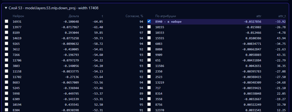
Why we rank by |t| rather than |μ|: some neurons have an enormous mean delta caused by two or three anomalous pairs. The t-statistic penalizes such dispersion. With a small number of pairs (fewer than 8), t is unreliable, so we fall back to ranking by |μ|.

3.3. From a million numbers to an image

Each layer is a vector of 17,408 mean deltas. For the heatmap, we create 128 bins by neuron index and take the mean within each bin. The result is a 64 × 128 matrix: layers vertically, bins horizontally, and color indicating the sign and magnitude of the delta. Separately, for each layer, the top-64 neurons by |t| are stored with their delta, t, and agreement—candidates for correction are later selected from them.

def bin_values(values, bin_count=128):"""Average of values across equal-width bins along the neuron index.""" totals = [0.0] * bin_count sizes = [0] * bin_count width = len(values) for index, value in enumerate(values): bucket = min(bin_count - 1, index * bin_count // width) totals[bucket] += float(value) sizes[bucket] += 1 return [totals[b] / sizes[b] if sizes[b] else 0.0 for b in range(bin_count)]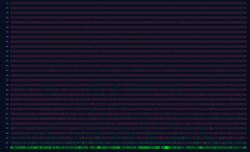

The first thing that caught my eye on the 1c_lang_query map: activation on incorrect answers is present in practically every layer. The model literally “pulls out” SQL-like constructs from the entire depth of the network. Hence, the practical conclusion that shaped the entire subsequent approach: we need not only strengthen the “good” neurons, but also suppress the erroneous ones!

Fig. 1

Fig. 2

Fig. 3

4. Attribution: which neuron actually influences the answer

Activation shows correlation, but not causality: a neuron may light up brightly on a rejected answer while having almost no influence on token selection. We need an assessment of the contribution to quality. As the target metric, we use margin—how much the model prefers the correct answer over the incorrect one on the differing tokens:

$\mathrm{margin}=\frac{1}{|T^c|}\sum_{t\in T^c}\log p(y_t\mid y_{<t})-\frac{1}{|T^r|}\sum_{t\in T^r}\log p(y_t\mid y_{<t})$

We calculate neuron attribution using the “gradient × input” method (first order of the Taylor series):

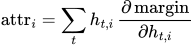
$\mathrm{attr}_i=\sum_t h_{t,i}\,\frac{\partial\,\mathrm{margin}}{\partial h_{t,i}}$

The meaning of the formula is: if the neuron’s activation is multiplied by m, then in the linear approximation the margin changes by

$\Delta\mathrm{margin}\approx(m-1)\,\mathrm{attr}_i$

This means that a neuron with attr < 0 reduces the margin through its activity—this is precisely an “erroneous” neuron. By damping it (m < 1), we expect the margin to increase.For a set of edits, the prediction is simply summed: Δmargin ≈ Σ (mᵢ − 1)·attrᵢ.

4.1. How to obtain the gradient with respect to the down_proj input

The trick is that the intermediate h is not a leaf of the graph, so autograd.grad cannot be computed directly on it after the forward pass. In the same pre-hook we replace the input with a leaf:

def hook(module, args): hidden = args[0] if not attribution_active: return None leaf = hidden.detach().requires_grad_(True) # new graph leaf leaves[name] = leaf return (leaf,) + tuple(args[1:]) # down_proj now computes from the leaf with torch.enable_grad(): out = model(input_ids=ids, attention_mask=mask, use_cache=False) objective = masked_mean_logprob(out.logits, ids, diff_rows) names = list(leaves) grads = torch.autograd.grad(objective * sign, [leaves[n] for n in names], allow_unused=True) attr = {} for name, grad in zip(names, grads): if grad is None: continue product = leaves[name].detach().float() * grad.float() attr[name] = product.reshape(-1, product.shape[-1]).sum(dim=0) # [17408]

For chosen, take sign = +1; for rejected, take sign = −1, and add them: this gives exactly the margin gradient. The mean log p function over the marked tokens accounts for the shift: token j is predicted by the logits at position j − 1:

def masked_mean_logprob(logits, input_ids, rows): positions = [i for i, flag in enumerate(rows) if flag and i > 0] if not positions: return None target = torch.tensor(positions, device=logits.device) picked = logits[0, target - 1].float() log_probs = torch.log_softmax(picked, dim=-1) tokens = input_ids[0, target].unsqueeze(-1)return log_probs.gather(-1, tokens).squeeze(-1).mean()

Attribution is expensive (a backward pass on a 27B model), so the map with attribution is built on a subsample: for 1c_lang_query — 512 pairs with a length of up to 2048 tokens. The map without attribution is built on all 2010 pairs. The mean and t are also calculated from the attribution, and the top-64 by |attr| are saved in the layer.

5. How to validate the edit

Attribution is only a prediction. The decision on each edit is made based on actual results on the held-out val split of the same dataset from which the map was built. For each pair, we calculate:

nll_chosen — the mean negative log p over the entire correct answer. Guard: the edit must not degrade the generation of the correct text overall;
margin — over the differing tokens, as in the attribution;
accuracy — the proportion of pairs with margin > 0.

To make the measurements comparable between runs, the val pairs are sorted by the query key (query_fingerprint, or sha1 of the last user message if it is absent). Separately, you can enable guard — several val pairs from other datasets — to ensure that the edit does not break neighboring skills. By default, guard is disabled: validation is performed strictly on the dataset used for the map.

During validation, the edit itself is applied “live” to the loaded BF16 model and is always rolled back:

def scale_columns(edits): """Multiplies the down_proj columns by edit["scale"] and returns the original values.""" saved = [] with torch.no_grad(): for edit in edits: weight = modules[edit["name"]].weight # [hidden, 17408] index = int(edit["index"]) saved.append((weight, index, weight[:, index].detach().clone())) weight[:, index].mul_(float(edit["scale"])) return saved def restore_columns(saved): with torch.no_grad(): for weight, index, column in saved: weight[:, index].copy_(column)

6. Multiplier modes

How to turn the selected neurons into specific multiplier coefficients m? There are four modes, with a strength parameter s ∈ [0, 1]:

Mode	Who is affected	Multiplier m
suppress (suppression)	only the erroneous ones: attr < 0, without attribution — Δ < 0	1 − s
sign	all selected, based on the sign of the activation delta	1 + s when Δ > 0, 1 − s when Δ < 0
attr	all selected, based on the sign of the attribution	1 + s when attr > 0, 1 − s when attr < 0
manual	all selected	a single number 0…2

After the experiment with 1c_lang_query, the default mode became suppress:suppress:boosting “good” neurons more often broke the NLL, while suppressing erroneous ones produced a sustained increase in the margin.

def signed_scales(edits, mode, value): result = [] for edit in edits: if mode == "suppress": source = edit.get("attr") if edit.get("attr") is not None else edit.get("delta") if source is None or source >= 0: continue # not erroneous — leave untouched scale = 1.0 - value elif mode == "manual": scale = value else: source = edit["delta"] if mode == "sign" else edit["attr"] scale = 1.0 + value if source > 0 else 1.0 - value if source < 0 else 1.0 result.append({**edit, "scale": max(0.0, min(2.0, scale))}) return result

7. Greedy selection with a control half

Taking the top 64 neurons and damping all of them at once is a bad idea: the edits interact, and the sum of linear predictions stops working. Therefore, the selection is greedy, one candidate at a time.

7.1. Splitting the validation set

The dataset’s validation pairs are split into two halves using a deterministic hash function of the request key: selection (where I make the decisions) and control (where I check the result). The same pair always falls into the same half.

def split_half(key: str) -> bool: """True — the pair is in the selection half, False — in the control half.""" return int(hashlib.sha1(key.encode("utf-8")).hexdigest()[-1], 16) % 2 == 0

7.2.Candidates and acceptance rule

Candidates are the top-N neurons by |attr| across all map layers (in suppress mode, only those with attr < 0), excluding those already accepted. Next, for each candidate: apply the edit on top of those already accepted, evaluate on the selection half, and keep or roll it back. Acceptance rule:

$\mathrm{margin}_{cand}>\mathrm{margin}_{cur}+\varepsilon\ \ \wedge\ \ \mathrm{nll}_{cand}\le\mathrm{nll}_{base}(1+\tau_{nll})$

By default, ε = 0.002 (per token), τ_nll = 2%, with a guard tolerance τ_guard = 1% for the nll and margin of each guard expert. Note that margin is compared against the current set (each accepted neuron must add value), whereas nll is compared against the baseline (degradations must not accumulate).

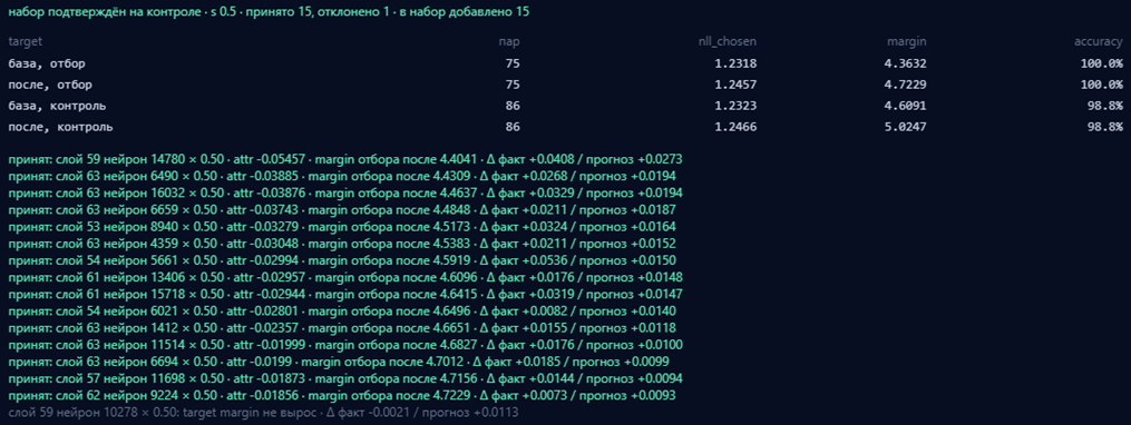
baseline = score(select, guard) # without edits current = baseline accepted, kept = [], [] for edit in signed_scales(candidates, mode, s): saved = scale_columns([edit]) summary = score(select, guard) ok, reason = greedy_accept(baseline, current, summary, eps, nll_tol, guard_tol) if ok: kept.extend(saved) # the edit remains in the weights current = summary accepted.append(edit) else: restore_columns(saved) final_control = score(control) # check the final result on the second half confirmed = accepted and passes(baseline_control, final_control) restore_columns(reversed(kept))

The set is considered confirmed only if margin increased on the control half and nll did not drop beyond the tolerance. This is the main safeguard against overfitting on val: greedy selection inevitably fits the noise in the sample on which it makes decisions.

Fig. 5

8.Hybrid mode: accumulating edits between runs

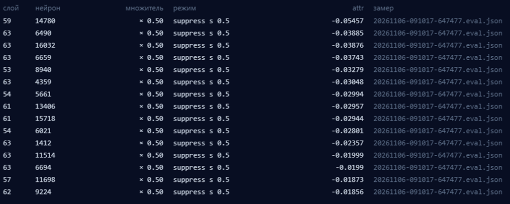
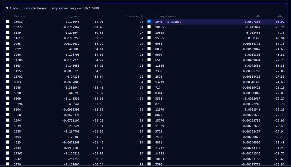
A single greedy selection run produces several dozen candidates. The idea is to rerun the selection in a different mode, with a different strength s, on the next candidates. To do this, each map has an edit set—a JSON file next to the map:

a new run starts on top of the set: the set’s edits are applied to the weights before the baseline is measured;
neurons in the set are excluded from the candidates;
accepted neurons are added to the set only if the run is confirmed on the control set;
a separate “entire set versus baseline” check shows the aggregate effect.

{ "schema_version": 1, "map": "20261105-125127-275881.json", "edits": [ {"name": "model.layers.54.mlp.down_proj", "layer_index": 54, "index": 5661, "attr": -0.0123, "scale": 0.5, "mode": "suppress", "s": 0.5, "eval": "20261106-072151-604012.eval.json"} ], "updated_at": "2026-11-06T07:31:02Z" }

The attr values in the example are illustrative.

9. Export: NERVE-GGUF

The final step is to export the modified model for inference in llama-server. The pipeline is as follows:

Editing the W_down columns is fully compatible with quantization: the quantizer simply sees slightly different weights. There are no additional layers, adapters, or inference-time hooks.

10. Results on 1c_lang_query

Example: how the model fails before the edit

One of the tasks in the public benchmarks for 1C.Prompt:

With a single query in the 1C query language, output all dates (by day) from the specified interval [&ДатаНачала; &ДатаОкончания] inclusively, sorted in ascending order. The interval is arbitrary (it may span several years) and is passed as parameters. The sequence of dates is built using query tools, without loops or processing the result in the module, and without using calendar tables from the configuration. In essence, this is a calendar in a query (a sequential list of dates for a specified period) without using pre-created metadata objects (such as a production calendar or schedule). In addition to the dates, it should output columns with the months, days of the week, and a calculated standard day off (Saturday and Sunday).

Model response before correction:

Solution: a recursive query (recursive CTE) in 1C:Enterprise 8.3. Starting with 8.3.17, the 1C query language has the РЕКУРСИВНО СОЕДИНИТЬ ВНЕШНЕ construct, which allows a sequence to be “expanded” directly in a query—without loops, calendar tables, or metadata objects.

The answer looks confident, but almost every key line in it is a hallucination:

A recursive CTE has been carried over from SQL. The 1C query language has no recursive queries, and “OUTER JOIN RECURSIVELY” and the reference to version 8.3.17 are made up. This is exactly the kind of transplantation of SQL constructs that can be seen in the heat map across all layers.
A nonexistent join. There is no “OUTER JOIN” in 1C—there are LEFT, RIGHT, FULL, and INNER JOIN, while results are combined using UNION (ALL).
Date arithmetic. In the query language, you cannot add a number to a date: to shift by one day, you need the ДОБАВИТЬКДАТЕ(Дата, ДЕНЬ, 1) function. In the built-in language, Date + 1 actually means plus one second.
Invented functions. МЕСЯЦ() and ДЕНЬНЕДЕЛИ() do exist, while МесяцНазвание() and ДеньНеделиНазвание() do not; names are obtained using CHOOSE … WHEN or FORMAT on the presentation side.
Broken package structure. ПОМЕСТИТЬ is in the middle of a construct, the temporary table references itself, and the package queries are not separated by semicolons—such text will not pass even syntax validation.

The correct solution is built without recursion: a temporary table of digits 0–9, its Cartesian product with itself produces a range of numbers N, and the dates are obtained as ДОБАВИТЬКДАТЕ(&ДатаНачала, ДЕНЬ, N), filtered by &ДатаОкончания.

The same prompt after the NERVE fix

SELECT&StartDate + (D1.Digit * 1000 + D2.Digit * 100 + D3.Digit * 10 + D4.Digit) AS Date, MONTH(&StartDate + (D1.Digit * 1000 + D2.Digit * 100 + D3.Digit * 10 + D4.Digit)) AS Month, WEEKDAY(&StartDate + (D1.Digit * 1000 + D2.Digit * 100 + D3.Digit * 10 + D4.Digit)) AS DayOfWeek, CASE WHEN WEEKDAY(&StartDate + (D1.Digit * 1000 + D2.Digit * 100 + D3.Digit * 10 + D4.Digit)) IN (6, 7) THEN TRUE ELSE FALSE END AS Weekend FROM (SELECT 0 AS Digit UNION ALL SELECT 1 UNION ALL SELECT 2 UNION ALL SELECT 3 UNION ALL SELECT 4 UNION ALL SELECT 5 UNION ALL SELECT 6 UNION ALL SELECT 7 UNION ALL SELECT 8 UNION ALL SELECT 9) AS D1, (SELECT 0 AS Digit UNION ALL SELECT 1 UNION ALL SELECT 2 UNION ALL SELECT 3 UNION ALL SELECT 4 UNION ALL SELECT 5 UNION ALL SELECT 6 UNION ALL SELECT 7 UNION ALL SELECT 8 UNION ALL SELECT 9) AS D2, (SELECT 0 AS Digit UNION ALL SELECT 1 UNION ALL SELECT 2 UNION ALL SELECT 3 UNION ALL SELECT 4 UNION ALL SELECT 5 UNION ALL SELECT 6 UNION ALL SELECT 7 UNION ALL SELECT 8 UNION ALL SELECT 9) AS D3, (SELECT 0 AS Digit UNION ALL SELECT 1 UNION ALL SELECT 2 UNION ALL SELECT 3 UNION ALL SELECT 4 UNION ALL SELECT 5 UNION ALL SELECT 6 UNION ALL SELECT 7 UNION ALL SELECT 8 UNION ALL SELECT 9) AS D4 WHERE D1.Digit * 1000 + D2.Digit * 100 + D3.Digit * 10 + D4.Digit <= DATEDIFF(&StartDate, &EndDate, DAY) ORDER BY Date

The difference is qualitative. The model has stopped inventing SQL constructs and returned to the idiom that 1C developers use to solve this task in practice:

No recursion or made-up syntax. Instead of a “recursive CTE”—a Cartesian product of four digit tables, 0–9, that is, a sequence of numbers 0…9999 (up to ~27 years—“a few years” with room to spare).
Only genuine query-language functions. DATADIFF(…, DAY) for the interval boundary, MONTH() and WEEKDAY() for the columns, CHOOSE … WHEN … IN (6, 7) for weekends—they all exist and are used as intended.
The right structure. One query, correctly nested UNION ALL, the condition in WHERE, and ordering by date. The interval is inclusive: when N = DATADIFF, &EndDate is output as well.

One error nevertheless remains: &StartDate + N. Date shifting in the query language is performed by the ADDDAY(&StartDate, DAY, N) function; adding a number to a date carries over a habit from the built-in language (where, moreover, +1 means one second, not one day). To make the query fully functional, it is sufficient to replace this expression in four places. It is telling that the error has shifted from the level of “the wrong language and an invented solution architecture” to the level of “one incorrect function”—exactly what should be expected from a targeted correction rather than retraining.

Example 2: query optimization—where edits are insufficient

The second prompt—“Optimize the query”—uses a fragment from the access management subsystem:

SELECT DISTINCT DefaultValues.AccessValueType AS ValueType,DefaultValues.AllAllowedWithoutExceptions AS AllAllowedWithoutExceptions INTO DefaultValuesForUser FROM InformationRegister.DefaultAccessGroupValues AS DefaultValues WHERE TRUE IN (SELECT TOP 1 TRUE FROM Catalog.AccessGroups.Users AS AccessGroupUsers INNER JOIN InformationRegister.UserGroupComposition AS UserGroupComposition ON AccessGroupUsers.Ref = DefaultValues.AccessGroup AND AccessGroupUsers.User = UserGroupComposition.UserGroup AND UserGroupComposition.User = &CurrentUser) ; SELECT DISTINCT DefaultValues.ValueType AS ValueType FROM DefaultValuesForUser AS DefaultValues GROUP BY DefaultValues.ValueType HAVING MIN(DefaultValues.AllAllowedWithoutExceptions) = TRUE

Model response before the edit:

SELECT DefaultValues.AccessValueType AS ValueType FROM InformationRegister.DefaultAccessGroupValues AS DefaultValues INNER JOIN Catalog.AccessGroups.Users AS AccessGroupUsers ON DefaultValues.AccessGroup = AccessGroupUsers.Ref INNER JOIN InformationRegister.UserGroupComposition AS UserGroupComposition ON AccessGroupUsers.User = UserGroupComposition.UserGroup AND UserGroupComposition.User = &CurrentUser GROUP BY DefaultValues.AccessValueType HAVING MIN(DefaultValues.AllAllowedWithoutExceptions) = TRUE

Model response after the NERVE correction:

// FIRST: get the current user's access groups SELECT DISTINCT AccessGroupUsers.Ref AS AccessGroup INTO UserAccessGroups FROM Catalog.AccessGroups.Users AS AccessGroupUsers INNER JOIN InformationRegister.UserGroupComposition AS UserGroupComposition ON AccessGroupUsers.Ref = UserGroupComposition.UserGroup AND UserGroupComposition.User = &CurrentUser ; // Index for the subsequent join CREATE INDEX UserAccessGroupIndex ON UserAccessGroups(AccessGroup) ; // SECOND: get default values for the user's groups SELECT DISTINCT DefaultValues.ValueType AS ValueType, DefaultValues.AllAllowedWithoutExceptions AS AllAllowedWithoutExceptions INTO DefaultValuesForUser FROM InformationRegister.AccessGroupDefaultValues AS DefaultValues INNER JOIN UserAccessGroups AS UserAccessGroups ON DefaultValues.AccessGroup = UserAccessGroups.AccessGroup ; // THIRD: get the value types for which all are allowed SELECT DISTINCT DefaultValuesForUser.ValueType AS ValueType FROM DefaultValuesForUser AS DefaultValuesForUser GROUP BY DefaultValuesForUser.ValueType HAVING MIN(DefaultValuesForUser.AllAllowedWithoutExceptions) = TRUE

This example shows more honestly than the first what the correction changes and what it does not.

What improved — the approach. The model before the correction simply “flattened” the subquery into a chain of joins: the result is the same, but the temporary table ЗначенияПоУмолчаниюДляПользователя disappeared (and it may be used further in the package), and instead of TOP 1, the join duplicates rows for each user group. The corrected model proposed a classic 1C optimization: calculate the user’s access groups once into a temporary table, index it, and replace the correlated subquery with a join — while preserving the original package contract.

What remained bad — accuracy. The corrected model’s response contains two errors:

Incorrect join field — critical. The original condition ГруппыДоступаПользователи.Пользователь = СоставыГруппПользователей.ГруппаПользователей became ГруппыДоступаПользователи.Ссылка = …ГруппаПользователей: an access group is compared with a user group, and the query will return an empty result.
Nonexistent index syntax. “CREATE INDEX … ON Table(Field)” is SQL. In 1C, an index on a temporary table is specified in the query itself: PUT ГруппыДоступаПользователя … INDEX BY ГруппаДоступа.

Conclusion: the correction based on the 1c_lang_query map moved the model toward the correct optimization idiom, but did not teach it to carry over join fields accurately, and one SQL reflex (CREATE INDEX) survived suppression.This is expected: a targeted edit removes specific “erroneous” directions in the activations, but does not add knowledge that the model does not have. Such cases are material for the next iteration: a new map based on pairs with connection errors, or for DPO.

11. Pitfalls and limitations

A single metric for the map and validation. Margin across the entire response versus margin across diff tokens—a difference of dozens of times. Any discrepancy in the mask between the map and validation makes the results incomparable.
Linear prediction works only for small edits. For m = 0 and for large sets, the observed fact noticeably diverges from Σ(m−1)·attr—so the decision is made solely based on the measurement.
Overfitting on the validation set. Greedy selection overfits to the sample. A holdout half is mandatory; I do not keep a set unless it is confirmed on the holdout.
Adjacent skills. Without a guard, an edit can spoil an adjacent dataset. If the expert domains overlap lexically (1C requests in natural language and in query language), it is worth enabling the guard.
Cost. A map with attribution over 512 pairs and greedy selection over dozens of candidates amounts to hours of GPU time on a 27B model. But it is still orders of magnitude cheaper than a new DPO cycle.
Truncation of long pairs. Pairs longer than max_length are truncated at the tail; if the difference lies beyond the boundary, the pair is dropped from the map.

Conclusions

A fine-tuned LLM is not a black box.A pair of simple tools—hooks on the down_proj input, pairwise statistics, and gradient attribution—provide a map showing which neurons pull the model toward error. A rigorous selection procedure with a held-out sample and a control half turns this map into a concrete, reproducible weight adjustment that goes into GGUF unchanged.

The main practical lesson with 1c_lang_query is that errors are “smeared” throughout the depth of the network, and it is more effective not only to strengthen the correct neurons but also suppress the erroneous neurons.

Adjusting just 15 neurons gave a significant boost to 1C query-language understanding!