How I Predicted Views on Habr Using ML / Habr

Data sampling and baseline metrics

To train the model, I needed a contrasting sample. I collected data on 80 other people’s articles from the “Freelance” hub on Habr (half from the recent feed and half from the best publications of all time) and added my own article with the label is_my_article = 1.The habr_dataset.csv table contained 81 records in total.

For each article, I collected basic structural parameters:

• title_length: title length in characters.

• word_count: total number of words in the text.

• images_count: number of images.

• TAG30@@links_count: number of links within the article.

• code_blocks_count: number of code blocks.

• views: article views converted from abbreviations such as 30K into regular integers.

Additionally, I saved the first 3000 characters of each text (text_preview) to submit them for analysis by a neural network.

How the local neural network copied the same answer 81 times in a row

Title length and the number of images alone are not enough because the algorithm does not understand the meaning of the text. Therefore, I wrote a script, ai_scorer.py, that sent the title and the beginning of each article to an LLM. The model was supposed to evaluate the text on a scale from 1 to 10 according to four criteria:

• clickbait_score: how attention-grabbing the title is.

• hook_score: how interestingly the introduction is written.

• pain_score: whether the topic addresses pressing issues (money, conflicts with clients, exchange commissions).

• readability_score: how easy the text is to read.

First, I tried to run the dataset through OpenRouter using the free model google/gemma-4-26b‑a4b‑it:free.On the very first article, the server returned a 429 error (temporarily rate-limited upstream) due to overload of the shared request pool.

Then I switched to running it locally. I have a Mac mini M4, so I used LM Studio to launch a local server with the quantized Qwen3 4B 2507 (MLX) model, weighing 2.12 GB.

The script quickly processed all 81 articles. But when I opened the terminal, I saw a strange result:

Every single one of the 81 articles received identical scores: Clickbait=7, Hook=6, Pain=8, Readability=7.

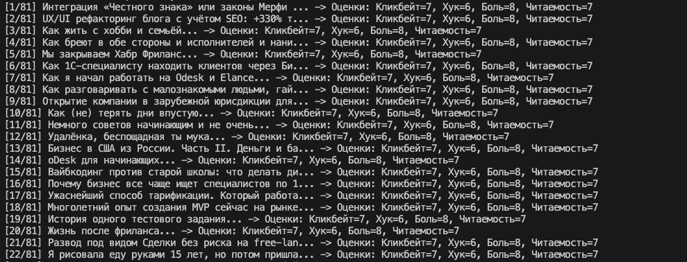
The problem turned out to be the prompt wording. At the end of the model’s instructions, I included an example of the correct JSON:

{"clickbait_score": 7, "hook_score": 6, "pain_score": 8, "readability_score": 7}

The small 4-billion-parameter model did not analyze the texts. It simply copied the numbers from my example for every article.If you feed such a column of identical numbers into a machine learning algorithm, it will be assigned zero importance.

Feature Engineering and Random Forest Training

To avoid depending on the hallucinations of a local model, I added a check for the uniqueness of scores (df['clickbait_score'].nunique() > 1) to the analysis script and wrote code to extract objective features from the text using regular expressions:

• has_question: whether the title contains a question mark.

• has_numbers: whether the title contains numbers.

• has_triggers: whether the title contains topic keywords (kwork, fl, upwork, деньг, рубл, обман, ошибк, заказчик, etc.).

• images_per_1000_words: how many images there are per 1,000 words of text.

Model training and article comparison code (ml_analyzer.py):

import re import numpy as np import pandas as pd from sklearn.ensemble import RandomForestRegressor df = pd.read_csv('habr_dataset_scored.csv') df['has_question'] = df['title'].apply(lambda x: 1 if '?' in str(x) else 0) df['has_numbers'] = df['title'].apply(lambda x: 1 if bool(re.search(r'\d', str(x))) else 0) trigger_words = ['kwork', 'fl', 'upwork', 'odesk', 'деньг', 'рубл', '$', 'обман', 'кидал', 'ошибк', 'устал', 'кладбище', 'жила', 'бизнес', 'заказчик'] df['has_triggers'] = df['title'].apply(lambda x: 1 if any(w in str(x).lower() for w in trigger_words) else 0) df['images_per_1000_words'] = (df['images_count'] / (df['word_count'] + 1)) * 1000 features = [ 'title_length', 'word_count', 'images_count', 'code_blocks_count', 'links_count', 'has_question', 'has_numbers', 'has_triggers', 'images_per_1000_words' ] X = df[features].fillna(0) y = np.log1p(df['views']) # Log-transform views to smooth out outliers model = RandomForestRegressor(n_estimators=200, random_state=42) model.fit(X, y) importances = pd.DataFrame({ 'Feature': features, 'Impact (%)': (model.feature_importances_ * 100).round(1) }).sort_values(by='Impact (%)', ascending=False) print(importances.to_string(index=False))

After running the script, it output the feature weights and compared my article’s parameters with the top 20% most popular publications in the sample (the threshold for inclusion was 148,000 views) and with weak articles (the bottom 40% of the sample, where average views were around 7,565):

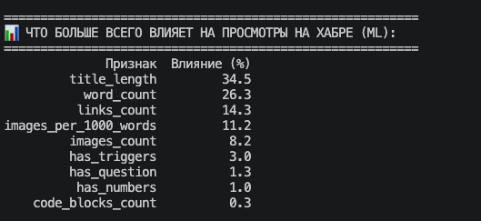
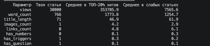
What do these figures show:

1. The title length (title_length) accounts for 34.5% of the influence. This is the main structural factor. Weak articles have an average title length of 61.9 characters. My article had a 71-character title (“Kwork — a graveyard for freelancers or a gold mine? Two sides of the same coin”). However, the average title length among the most-read articles in the top 20% is 46.9 characters. Shorter titles are read more easily in the feed. If I remove the second part (“Two sides of the same coin”) from my title, exactly 46 characters will remain.

2. The article length (word_count) accounts for 26.3% of the influence. My article had only 766 words. Weak articles have an average of 1,254.7 words, while the average length in the top 20% is 1,773.8 words.Long-form longreads receive more reading time and rank better in search.

3. Links and images (links_count, images_per_1000_words, images_count) collectively account for 33.7% of the influence. Top-performing posts average 4.2 images and 4.8 links. My article had only one cover image and no links.

4. Code blocks (code_blocks_count) affect only 0.3%. For a hub about freelancing, this makes sense: the audience comes there for analyses of work situations and personal experiences, not for code snippets.

A data leakage error when creating the predictor

At the next step, I decided to write a predictor.py script that would predict the success of a new article before its publication. I set the “hit” threshold at 25,000 views and trained two models: RandomForestClassifier (estimates the probability of surpassing 25K views as a percentage) and RandomForestRegressor (predicts the expected number of views).

To test this, I ran two variants through the model:

1. The original parameters of my article (a 71-character headline, 766 words, 1 image, 0 links).

2. A revised version based on the metrics of top posts (a short headline with a number, 1,750 words, 5 images, 4 links).

Unexpectedly, the first (raw) version had a higher probability of success than the revised second version.

When analyzing the code, I found that I had made two mistakes:

1. Data Leakage (data leakage). My article (which already had 30,000 views, above the threshold of 25,000) remained in the training set.Decision trees without a depth limit simply memorized the specific combination (71 characters + 766 words = more than 25K views). When I submitted the same figures to the test, the algorithm produced an inflated estimate because it had already seen this example during training.

2. Penalty for digits in the title. In the second test version, I added a digit to the title. According to our table, digits appeared in the titles of weak articles three times more often (0.3) than in top articles (0.1), due to the large number of advertising cases in the fresh feed.

I fixed the script: I excluded my own article from the training sample (train_df = df[df['is_my_article'] == 0]) and limited the depth of the trees using the max_depth=4 parameter so that the model would look for general rules rather than memorize individual rows.

The result of the honest test:

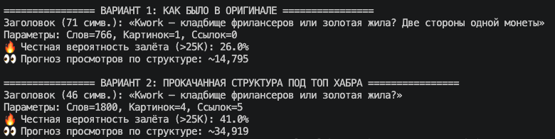
Now the metrics made sense. My original article (which the model had not seen before) received, solely because of its structure, a 26.0% probability of gaining more than 25,000 views and a baseline forecast of 14,795 views.
The second version, with an improved structure (46-character title, 1,800 words, 4 images, 5 links), received a 41.0% probability and a forecast of 34,919 views.

Why did the model predict 14,795 views when the actual result was 30,000?

This reveals the main limitation of the structural model. The algorithm evaluated only the “packaging” of the text: title length, word count, and the presence of images and links.He did not know what exactly the article was about.

For a short article of 766 words with one image and a long headline, 14.8 thousand views is a normal average ceiling. The article actually got 30,000 views (twice the forecast) because of the topic of the Kwork marketplace itself and the discussion of earnings in the comments.

But this leads to a practical conclusion: if a hot topic by itself doubles the reach, then packaging the same material into a full-fledged longread (1,800 words with 4 images and a short headline) would already push the baseline to around 35,000 views, while the final reach could exceed 60,000.

Final script for testing drafts

In the end, I removed the test stubs from predictor.py and created a console utility with manual parameter entry via input().

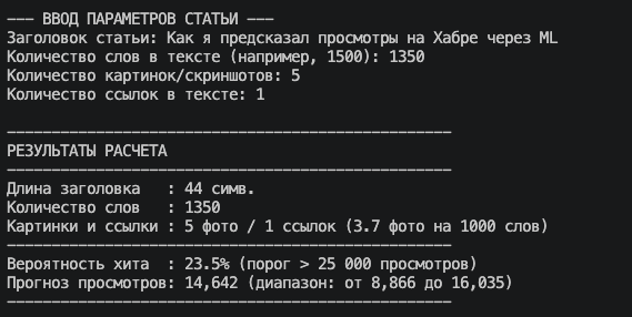
To avoid relying on a single averaged figure, I added a calculation of the interquartile range (IQR—the range between the 25th and 75th percentiles of the predictions from all 200 individual trees within RandomForestRegressor). This makes it possible to see the minimum and maximum range of views for the selected article structure:

import numpy as np import pandas as pd from sklearn.ensemble import RandomForestRegressor, RandomForestClassifier def build_models(csv_path='habr_dataset_scored.csv'): df = pd.read_csv(csv_path) train_df = df[df['is_my_article'] == 0].copy() features = ['title_length', 'word_count', 'images_count', 'links_count', 'images_per_1000_words'] train_df['images_per_1000_words'] = (train_df['images_count'] / (train_df['word_count'] + 1)) * 1000 X_train = train_df[features].fillna(0) y_views = np.log1p(train_df['views'])y_hit = (train_df['views'] >= 25000).astype(int) reg = RandomForestRegressor(n_estimators=200, max_depth=4, random_state=42).fit(X_train, y_views) clf = RandomForestClassifier(n_estimators=200, max_depth=4, random_state=42).fit(X_train, y_hit) return reg, clf, features

Here are the predictions for this article:

Conclusions based on the figures

If we use the model’s data for non-technical and career-oriented publications as a benchmark:

1. A headline of around 45–50 characters. Long, two-sentence structures reduce click-through rates in feeds.

2. Text length of 1,500–1,800 words. Short articles under 800 words perform worse in terms of audience retention and search traffic.

3. At least 4 illustrations and 4–5 links. Graphics break up the text canvas (the optimal density is about 2.5 images per 1,000 words).

4. Data validation after using the LLM. Small local models require strict response validation; otherwise, they easily copy examples directly from the system prompt.

This article has already been written taking into account the parameters produced by the script.Let's see in practice whether the actual number of views matches the model's estimated range.